ppm

ppmpy.ppm

PPM is a Python module for reading Yprofile-01-xxxx.bobaaa files as well as some analysis involving Rprofile files and Mesa stellar models.

Simple session for working with ppmpy, here I assume user’s working on

astrohub

which is the intended environment for ppmpy.

If the user find any bugs or errors, please email us.

Examples

Here is an example runthrough.

In [1]: from ppmpy import ppm
   ...: !ls /data/ppm_rpod2/YProfiles/
   ...: 
AGBTP_M2.0Z1.e-5  O-shell-M25	  agb-entrainment-convergence
C-ingestion	  O-shell-mixing  sakurai
M4ZAMS		  RAWD		  sakurai-num-exp-robustness-onset-GOSH

In [3]: data_dir = '/data/ppm_rpod2/YProfiles/'
   ...: project = 'O-shell-M25'
   ...: ppm.set_YProf_path(data_dir+project)
   ...: 

In [6]: ppm.cases
Out[6]: 
['D10',
 'D11',
 'D14',
 'D23',
 'D17',
 'D4',
 'D24b',
 'D1_toomuchoutput',
 'D5',
 'D3',
 'D9',
 'D26',
 'D22',
 'D19',
 'D15',
 'D16',
 'D28',
 'D27',
 'D8',
 'D1',
 'D18',
 'D6',
 'D12',
 'D25',
 'D20',
 'D24a',
 'D21',
 'D2']

and

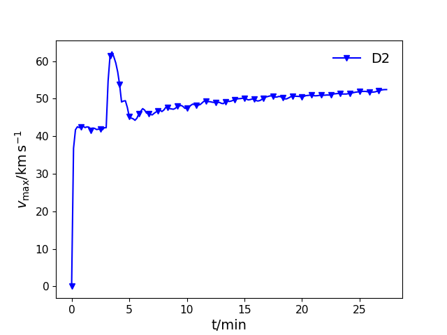
In [7]: D2=ppm.yprofile('D2')
   ...: D2.vprofs(100)
   ...: 

plots the data.

(Source code, png, hires.png, pdf)

Functions

L_H_L_He_comparison(cases[, sparse, ifig, …])	Compares L_H to L_He, optional values are set to values from O-shell burning paper.
analyse_dump(rp, r1, r2)	This function analyses ray profiles of one dump and returns
bucket_map(rprofile, quantity[, limits, …])	Plots a Mollweide projection of the rprofile object using the mpl_toolkits.basemap package
cdiff(x)
cmap_from_str(str[, segment])
colourmap_from_str(str[, segment])
compare_entrained_material(yps, labels, fname)	Compares the entrainment rate of two seperate yprofile objects
energy_comparison(yprof, mesa_model[, …])	Nuclear energy generation rate (enuc) thermal neutrino
get_N2(yp, dump)	squared Brunt-Vaisala frequency N^2
get_avg_rms_velocities(prof, dumps, comp)	Finds an average velocity vector as a function of radius for a given range of dumps.
get_heat_source(yprof[, radbase, dlayerbot, …])	returns estimation of yprofiles energy
get_mach_number(rp_set, yp, dumps, comp[, …])	Returns max Mach number and matching time vector
get_mesa_time_evo(mesa_path, mesa_logs, t_end)	Function to generate data for figure 5 in O-shell paper.
get_p_top(prof, dumps, r_top)	Returns p_top and matching time vector
get_power_spectrum_RProfile(yprof_path, …)	Calculates power spectra of radial velocity
get_r_int(data_path, r_ref, gamma[, sparse])	Returns values for radius of interface for a given reference radius.
get_upper_bound(data_path, r1, r2[, sparse])	Returns information about the upper convective boundary
get_v_evolution(prof, cycles, r1, r2, comp, RMS)	Finds a velocity vector and a time vector for a range of cycles
luminosity_for_dump(path[, get_t])	Takes a directory and returns luminosity and time vector with entry
make_colourmap(colours[, alphas])	make a matplotlib colormap given a list of index [0-255], RGB tuple values
plot_Mollweide(rp_set, dump_min, dump_max, …)	Plot Mollweide spherical projection plot
plot_N2(case, dump1, dump2, lims1, lims2, …)	plots squared Brunt-Vaisala frequency N^2 with zoom window
plot_boundary_evolution(data_path, r1, r2[, …])	Displays the time evolution of the convective boundary or Interface radius
plot_diffusion_profiles(run, mesa_path, …)	This is a function that generates various diffusion profiles
plot_entr_v_ut(cases, c0, Ncycles, r1, r2, …)	Plots entrainment rate vs max radial or tangential velocity.
plot_luminosity(L_H_yp, L_H_rp, t)	Plots two luminosity vectors against the same time vector
plot_mach_number(rp_set, yp, dumps[, comp, …])	A function for geterating the time evolution of the mach number.
plot_mesa_time_evo(mesa_path, mesa_logs, t_end)	Function to plot data for figure 5 in O-shell paper.
plot_p_top(yp, dumps, r_top[, ifig, lims, …])	param yp:
plot_power_spectrum_RProfile(t, l, power[, …])	Plots power spectra of radial velocity
prep_Yprofile_data([user, run])	for given user and run create YProfile dir in run dir and link all
prof_compare(cases[, ndump, yaxis_thing, …])	Compare profiles of quantities from multiple PPM Yprofile instances at a given time of nump number.
set_YProf_path(path[, YProf_fname])	Set path to location where YProfile directories can be found.
set_nice_params()
upper_bound_ut(data_path, dump_to_plot, …)	Finds the upper convective boundary as defined by the steepest decline in tangential velocity.
v_evolution(cases, ymin, ymax, comp, RMS[, …])	Compares the time evolution of the max RMS velocity of different runs

Classes

LUT(lutfile, p0, p1, s0, s1[, posdef])
yprofile([sldir, filename_offset, silent])	Data structure for holding data in the YProfile.bobaaa files.

ppmpy.ppm.L_H_L_He_comparison(cases, sparse=1, ifig=101, L_He=0.006713640000000001, airmu=1.39165, cldmu=0.725, fkair=0.203606102635, fkcld=0.885906040268, AtomicNoair=6.65742024965, AtomicNocld=1.34228187919, markevery=1, lims=None, save=False)

Compares L_H to L_He, optional values are set to values from O-shell burning paper.

Parameters:

• cases (string array) – names of yprofile instances i.e[‘D1’,’D2’…]
• sparse (int) – what interval in the range to calculate 1 calculates every dump 2 every second dump ect
• lims (array) – plot limits
• save (boolean) – save figure

class ppmpy.ppm.Messenger(verbose=3)

Messenger reports messages, warnings, and errors to the user.

error(error)

Reports an error to the user. The error is currently printed to stdout.

Parameters:error (string) –

message(message)

Reports a message to the user. The message is currently printed to stdout.

Parameters:message (string) –

warning(warning)

Reports a warning to the user. The warning is currently printed to stdout.

Parameters:warning (string) –

class ppmpy.ppm.Rprof(file_path, verbose=3)

Rprof reads and holds the contents of a single .rprof file written by PPMstar 2.0.

get(var, resolution='l')

Returns variable var if it exists. The method first searches for a variable name match in this order: header variables, low- resolution variables, and high-resolution variables.

Parameters:

• var (string) – Variable name.
• resolution (string (case insensitive)) – ‘l’ (low) or ‘h’ (high). A few variables are available at double resolution (‘h’), the rest correspond to the resolution of the computational grid (‘l’).

Returns:

Return type:

Variable var, if found.

get_header_variables()

Returns a list of header variables available.

get_hr_variables()

Returns a list of high-resolution variables available.

get_lr_variables()

Returns a list of low-resolution variables available.

is_valid()

Checks if the instance is valid, i.e. fully initialised.

Returns: Return type:True if the instance is valid. False otherwise.

class ppmpy.ppm.RprofHistory(file_path, verbose=3)

RprofHistory reads .hstry files produced by PPMstar 2.0.

get(var_name)

Returns variable var_name if it exists.

Parameters:var_name (string) – Returns:

• Variable as a numpy array or None if var_name is not
• a valid variable name.

get_variables()

Returns a list of variables available.

is_valid()

Checks if the instance is valid, i.e. fully initialised.

Returns: Return type:True if the instance is valid. False otherwise.

plot_wct_per_dump()

Plots wall-clock time (WCT) per dump as a function of dump number.

class ppmpy.ppm.RprofSet(dir_name, verbose=3)

RprofSet holds a set of .rprof files from a single run of PPMstar 2.0.

get(var, fname, num_type='NDump', resolution='l')

Returns variable var at a specific point in the simulation’s time evolution.

Parameters:

• var (string) – Name of the variable.
• fname (integer/float) – Dump number or time in seconds depending on the value of num_type.
• num_type (string (case insensitive)) – If ‘ndump’ fname is expected to be a dump number (integer). If ‘t’ fname is expected to be a time value in seconds; run history file (.hstry) must be available to search by time value.
• resolution (string (case insensitive)) – ‘l’ (low) or ‘h’ (high). A few variables are available at double resolution (‘h’), the rest correspond to the resolution of the computational grid (‘l’).

Returns:

• Variable var as given by Rprof.get() if the Rprof corresponding to
• fname exists and None otherwise.

get_dump(dump)

Returns a single dump.

Parameters:dump (integer) –

get_dump_list()

Returns a list of dumps available.

get_history()

Returns the RprofHistory object associated with this instance if available and None otherwise.

get_run_id()

Returns the run identifier that precedes the dump number in the names of .rprof files.

is_valid()

Checks if the instance is valid, i.e. fully initialised.

Returns: Return type:True if the instance is valid. False otherwise.

ppmpy.ppm.analyse_dump(rp, r1, r2)

This function analyses ray profiles of one dump and returns

r, ut, dutdr, r_ub,

Parameters:

• rp (radial profile) – radial profile
• r1 (float) – minimum radius for the search for r_ub
• r2 (float) – maximum radius for the search for r_ub

Returns:

• r (array) – radius
• ut (array) – RMS tangential velocity profiles for all buckets (except the 0th)
• dutdr (array) – radial gradient of ut for all buckets (except the 0th)
• r_ub (array) – radius of the upper boundary as defined by the minimum in dutdr for all buckets (except the 0th).

ppmpy.ppm.bucket_map(rprofile, quantity, limits=None, ticks=None, file_name=None, time=None)

Plots a Mollweide projection of the rprofile object using the mpl_toolkits.basemap package

Parameters:

• rprofile (rprofile object) – rprofile dump used just for geometry
• quantity (array) – data to be passed into the projection
• limits (2 index array) – cmap limits, scale the colormap for limit[0] =min to limit[1] =max
• ticks – passed into matplotlib.colors.ColorbarBase see ColourbarBase
• file_name (string) – file name: ‘/path/filename’ to save the image as
• time (float) – time to display as the title

ppmpy.ppm.compare_entrained_material(yps, labels, fname, ifig=1)

Compares the entrainment rate of two seperate yprofile objects

Parameters:

• yps (yprofile objects) – yprofiles to compare
• labels (string array matching yp array) – labels for yp objects
• fname – specific dump to access information from

Examples

import ppm yp1 = yprofile(‘/data/ppm_rpod2/YProfiles/agb-entrainment-convergence/H1’) yp2 = yprofile(‘/data/ppm_rpod2/YProfiles/O-shell-M25/D2’) compare_entrained_material([yp1,yp2],[‘O shell’,’AGB’], fname = 271)

ppmpy.ppm.energy_comparison(yprof, mesa_model, xthing='m', ifig=2, silent=True, range_conv1=None, range_conv2=None, xlim=[0.5, 2.5], ylim=[8, 13], radbase=4.1297, dlayerbot=0.5, totallum=20.153)

Nuclear energy generation rate (enuc) thermal neutrino energy loss rate (enu) and luminosity profiles (L) for MESA plotted with ppmstar energy estimation (eppm)

Parameters:

• yprof (yprofile object) – yprofile to examine
• mesa_model (mesa_model) – mesa model to examine
• xthing (str) – x axis as mass, ‘m’ or radius, ‘r’
• silent (bool) – suppress output or not
• range_conv1 (range, optional) – range to shade for convection zone 1
• range_conv2 (range, optional) – range to shade for convection zone 2
• xlim (range) –
• ylim (range) –
• from setup.txt (values) –
• = 4.1297 (radbase) –
• = 0.5 (dlayerbot) –
• = 20.153 (totallum) –

Examples

import ppm import nugrid.mesa as ms mesa_A_model_num = 29350 mesa_logs_path = ‘/data/ppm_rpod2/Stellar_models/O-shell-M25/M25Z0.02/LOGS_N2b’ mesa_model = ms.mesa_profile(mesa_logs_path, mesa_A_model_num) yprof = yprofile(‘/data/ppm_rpod2/YProfiles/O-shell-M25/D1’) energy_comparison(yprof,mesa_model)

ppmpy.ppm.get_N2(yp, dump)

squared Brunt-Vaisala frequency N^2

Parameters:

• = yprofile object (yp) – yprofile to use
• = int (dump) – dump to analyze

Returns:

Brunt Vaisala frequency [rad^2 s^-1]

Return type:

N2 = vector

ppmpy.ppm.get_avg_rms_velocities(prof, dumps, comp)

Finds an average velocity vector as a function of radius for a given range of dumps. To find a velocity vector as a function of radius see get_v_evolution().

Parameters:

• yprof (yprofile instance) – profile to examine
• dumps (range) – dumps to average over
• comp (string) – component to use ‘r’:’radial’,’t’:’tangential’,’tot’:’total’

ppmpy.ppm.get_heat_source(yprof, radbase=4.1297, dlayerbot=0.5, totallum=20.153)

returns estimation of yprofiles energy

# values from setup.txt radbase = 4.1297 dlayerbot = 0.5 totallum = 20.153

Parameters:yprof (yprofile object) – yprofile to examine Returns:array with vectors [radius, mass, energy estimate] Return type:array

ppmpy.ppm.get_mach_number(rp_set, yp, dumps, comp, filename_offset=1)

Returns max Mach number and matching time vector

Parameters:

• yp (yprofile instance) –
• rp_set (rprofile set instance) –
• dumps (range) – range of dumps to include
• comp (string) – ‘mean’ ‘max’ or ‘min’ mach number

Returns:

• Ma_max (vector) – max mach nunmber
• t (vector) – time vector

ppmpy.ppm.get_mesa_time_evo(mesa_path, mesa_logs, t_end, save=False)

Function to generate data for figure 5 in O-shell paper.

Parameters:

• mesa_path (string) – path to the mesa data
• mesa_logs (range) – cycles you would like to include in the plot
• t_end (float) – time of core collapse
• save (boolean,optional) – save the output into data files

Returns:

• agearr (array) – age yrs
• ltlarr (array) – time until core collapse
• rbotarr (array) – radius of lower convective boundary
• rtoparr (array) – radius of top convective boundary
• muarr (array) – mean molecular weight in convective region
• peakLarr (array) – peak luminosity
• peakL_Lsunarr (array) – peak luminosity units Lsun
• peakepsgravarr (array) – peak sepperation

ppmpy.ppm.get_p_top(prof, dumps, r_top)

Returns p_top and matching time vector

Parameters:

• yp (yprofile instance) –
• rtop (float) – boundary radius
• dumps (range) – range of dumps to include can be sparse

Returns:

• Ma_max (vector) – max mach nunmber
• t (vector) – time vector

ppmpy.ppm.get_power_spectrum_RProfile(yprof_path, rprof_path, r0, t_lim=None, t_res=None, l_max=6)

Calculates power spectra of radial velocity

Parameters:

• yprof_path/rprof_path (strings) – paths for matching rprofile and yprofile files
• r0 (float) – radius to examine
• t_lim (2 index array) – [t_min, t_max], data to look at
• t_res (int) – set number of data points between [t_min, t_max], None = ndumps
• l_max – maximum spherical harmonic degree l

Returns:

t,l,power

Return type:

time, spherical harmonic degree l, and power vectors

ppmpy.ppm.get_r_int(data_path, r_ref, gamma, sparse=1)

Returns values for radius of interface for a given reference radius.

Parameters:

• data_path (string) – data path
• r_ref (float) – r_int is the radius of the interface at which the relative [A(t) - A0(t)]/A0(t) with respect to a reference value A0(t) exceeds a threshold. The reference value A0(t) is taken to be the average A at a reference radius r_ref at time t. We need to put r_ref to the bottom of the convection zone, because most of the convection zone is heated in the final explosion. The threshold should be a few times larger than the typical bucket-to-bucket fluctuations in A due to convection. A value of 1e-3 is a good trade-off between sensitivity and the amount of noise.
• sparse (int, optional) – What interval to have between data points

Returns:

• [all arrays]
• avg_r_int (average radius of interface)
• sigmam_r_int/sigmap_r_int (2 sigma fluctuations in r_int)
• r_int (interface radius)
• t (time)

ppmpy.ppm.get_upper_bound(data_path, r1, r2, sparse=10)

Returns information about the upper convective boundary

Parameters:

• data_path (string) – path to rprofile set
• = float (r1/r2) – This function will only search for the convective boundary in the range between r1/r2
• sparse (int) – What interval to plot data at

Returns:

• [all arrays]
• avg_r_ub (average radius of upper boundary)
• sigmam_r_ub/sigmap_r_ub (2 sigma fluctuations in upper boundary)
• r_ub (upper boundary)
• t (time)

ppmpy.ppm.get_v_evolution(prof, cycles, r1, r2, comp, RMS)

Finds a velocity vector and a time vector for a range of cycles

Parameters:

• prof (yprofile object) – prof to look at
• cycles (range) – cycles to look at
• r1/r1 (float) – boundaries of the range to look for v max in
• comp (string) – velocity component to look for ‘radial’ or ‘tangential’
• RMS (string) – ‘mean’ ‘min’ or ‘max velocity

ppmpy.ppm.luminosity_for_dump(path, get_t=False)

Takes a directory and returns luminosity and time vector with entry corresponding to each file in the dump

!Can take both rprofile and yprofile filepaths

Parameters:

• path (string) – Filepath for the dumps, rprofile or yprofile dumps.
• get_t (Boolean) – Return the time vector or not

Returns:

• t (1*ndumps array) – time vector [t/min]
• L_H (1*ndumps array) – luminosity vector [L/Lsun]

ppmpy.ppm.make_colourmap(colours, alphas=None)

make a matplotlib colormap given a list of index [0-255], RGB tuple values (normalised 0-1) and (optionally) a list of alpha index [0-255] and alpha values, i.e.:

colours = [[0, (0., 0., 0.)], [1, (1., 1., 1.)]] alphas = [[0, 0.], [1, 1.]]

ppmpy.ppm.plot_Mollweide(rp_set, dump_min, dump_max, r1, r2, output_dir=None, Filename=None, ifig=2)

Plot Mollweide spherical projection plot

Parameters:

• = int (dump_min/dump_max) – Range of file numbers you want to use in the histogram
• = float (r1/r2) – This function will only search for the convective boundary in the range between r1/r2
• ouput_dir (string) – path to output directory
• filename (string) – name for output file, None: no output

Examples

data_path = “/rpod2/PPM/RProfiles/AGBTP_M2.0Z1.e-5/F4” rp_set = rprofile.rprofile_set(data_path) plot_Mollweide(rp_set, 100,209,7.4,8.4)

ppmpy.ppm.plot_N2(case, dump1, dump2, lims1, lims2, mesa_logs_path, mesa_model_num)

plots squared Brunt-Vaisala frequency N^2 with zoom window

Parameters:

• = string (case) – Name of run eg. ‘D1’
• dump2 = int (dump1/) – dump to analyze
• = int (mesa_A_model_num) – number for mesa model
• = 4 index array (lims1/lims2) – axes limits [xmin xmax ymin ymax] lims1 = smaller window

Examples

import ppm set_YProf_path(‘/data/ppm_rpod2/YProfiles/O-shell-M25/’) plot_N2(‘D1’, 0, 132, mesa_model_num = 29350, mesa_B_model_num = 28950)

ppmpy.ppm.plot_boundary_evolution(data_path, r1, r2, t_fit_start=700, silent=True, show_fits=False, ifig=5, r_int=False, r_ref=None, gamma=None, sparse=10, lims=None, insert=False)

Displays the time evolution of the convective boundary or Interface radius

Plots Fig. 14 or 15 in paper: “Idealized hydrodynamic simulations of turbulent oxygen-burning shell convection in 4 geometry” by Jones, S.; Andrassy, R.; Sandalski, S.; Davis, A.; Woodward, P.; Herwig, F. NASA ADS: http://adsabs.harvard.edu/abs/2017MNRAS.465.2991J

Parameters:

• data_path (string) – data path
• r1/r2 (float) – This function will only search for the convective boundary in the range between r1/r2
• show_fits (boolean, optional) – show the fits used in finding the upper boundary
• t_fit_start (int) – The time to start the fit for upper boundary fit takes range t[t_fit_start:-1] and computes average boundary
• r_int (bool, optional) – True plots interface radius, False plots convective boundary !If true r_ref must have a value
• r_ref (float) – r_int is the radius of the interface at which the relative [A(t) - A0(t)]/A0(t) with respect to a reference value A0(t) exceeds a threshold. The reference value A0(t) is taken to be the average A at a reference radius r_ref at time t. We need to put r_ref to the bottom of the convection zone, because most of the convection zone is heated in the final explosion. The threshold should be a few times larger than the typical bucket-to-bucket fluctuations in A due to convection. A value of 1e-3 is a good trade-off between sensitivity and the amount of noise.
• sparse (int, optional) – What interval to have between data points
• lims (array) – limits of the insert axes [xl,xu,yl,yu]
• insert (bool) – whether or not to include a second inserted subplot

ppmpy.ppm.plot_diffusion_profiles(run, mesa_path, mesa_log, rtop, Dsolve_range, tauconv, r0, D0, f1, f2, alpha, fluid='FV H+He', markevery=25)

This is a function that generates various diffusion profiles it is dependant on the functions Dsolvedown and Dov2

Parameters:

• run (string) – yprofile case to use i.e. ‘D2’
• mesa_path (string) – path to the mesa data
• mesa_logs (range) – cycles you would like to include in the plot
• Dsolve_range (int array) – cycles from which to take initial and final abundance profiles for the diffusion step we want to mimic.
• fluid (string) – Which fluid do you want to track?
• tauconv (float, optional) – If averaging the abundance profiles over a convective turnover timescale, give the convective turnover timescale (seconds). The default value is None.
• r0 (float) – radius (Mm) at which the decay will begin
• D0 (float) – diffusion coefficient at r0
• f1,f2 (float) – parameters of the model

Examples

plot_diffusion_profiles(‘D2’,’/data/ppm_rpod2/Stellar_models/O-shell-M25/M25Z0.02/’,28900,

7.8489,(1,160),2.*460.,7.8282,10.**12.27,0.21,0.055,1.6)

pl.xlim(3,9) pl.ylim(11,16)

ppmpy.ppm.plot_entr_v_ut(cases, c0, Ncycles, r1, r2, comp, metric, label, ifig=3, integrate_both_fluids=False)

Plots entrainment rate vs max radial or tangential velocity.

Parameters:

• cases (string list) – list of cases i.e.D1
• c0 (list) – cycle to start on for each case
• Ncycles (int) – number of cycles to average to find v
• r1 (float) – radius range to search for v, also r2
• comp (str) – component of velocity ‘tangential’ or ‘radial’
• metric (str) – metric of veloctiy ‘min’ max’ or ‘mean’

Examples

cases = (‘D1’, ‘D8’, ‘D5’, ‘D6’, ‘D9’, ‘D10’, ‘D20’, ‘D23’, ‘D2’) c0 = (241,154,142,155,123,78,355,241,124) global ppm_path ppm_path = ‘/data/ppm_rpod2/YProfiles/O-shell-M25/’ plot_entr_v_ut(cases,c0,10,7.5,8.5,ifig = 3,integrate_both_fluids = False)

ppmpy.ppm.plot_luminosity(L_H_yp, L_H_rp, t)

Plots two luminosity vectors against the same time vector

Parameters:

• L_H_yp (1 *ndumps vector) – Luminosity vector for yprofile can be generated by luminosity_for_dump
• L_H_rp (1 *ndumps vector) – Luminosity vector for rprofile can be generated by luminosity_for_dump
• t (array size(L_H_rp)) – time vector to be plotted on the x-axis

ppmpy.ppm.plot_mach_number(rp_set, yp, dumps, comp='max', ifig=1, lims=None, insert=False, save=False, prefix='PPM', format='pdf', lims_insert=None, f_offset=1)

A function for geterating the time evolution of the mach number.

Parameters:

• yp (yprofile instance) –
• rp_set (rprofile set instance) –
• dumps (range) – range of dumps to include
• lims (list) – Limits for the plot, i.e. [xl,xu,yl,yu]. If None, the default values are used. The default is None.
• save (boolean) – Do you want the figures to be saved for each cycle? Figure names will be <prefix>-Vel-00000000001.<format>, where <prefix> and <format> are input options that default to ‘PPM’ and ‘pdf’. The default value is False.
• prefix (string) – see ‘save’ above
• format (string) – see ‘save’ above

ppmpy.ppm.plot_mesa_time_evo(mesa_path, mesa_logs, t_end, ifig=21)

Function to plot data for figure 5 in O-shell paper.

Parameters:

• mesa_path (string) – path to the mesa data
• mesa_logs (range) – cycles you would like to include in the plot
• t_end (float) – time of core collapse
• save (boolean, optional) – save the output into data files

Examples

plot_mesa_time_evo(‘/data/ppm_rpod2/Stellar_models/O-shell-M25/M25Z0.02/LOGS’,

range(550,560),7.5829245098141646E+006,ifig=21)

ppmpy.ppm.plot_p_top(yp, dumps, r_top, ifig=1, lims=None, insert=False, save=False, prefix='PPM', format='pdf', lims_insert=None)

Parameters:

• yp (yprofile instance) –
• r_top (float) – boundary radius
• dumps (range) – range of dumps to include can be sparse
• lims (list) – Limits for the plot, i.e. [xl,xu,yl,yu]. If None, the default values are used. The default is None.
• save (boolean) – Do you want the figures to be saved for each cycle? Figure names will be <prefix>-Vel-00000000001.<format>, where <prefix> and <format> are input options that default to ‘PPM’ and ‘pdf’. The default value is False.
• prefix (string) – see ‘save’ above
• format (string) – see ‘save’ above

ppmpy.ppm.plot_power_spectrum_RProfile(t, l, power, ifig=1, title='', vmin=0.01, vmax=1.0)

Plots power spectra of radial velocity

Parameters:

• t,l,power (arrays) – time, sperical harmonic degree and power generated by get_power_spectrum_RProfile()
• title (string) – title

ppmpy.ppm.prep_Yprofile_data(user='Paul', run='BW-Sakurai-1536-N13')

for given user and run create YProfile dir in run dir and link all YProfile data from dump directories

this is for use on BlueWaters

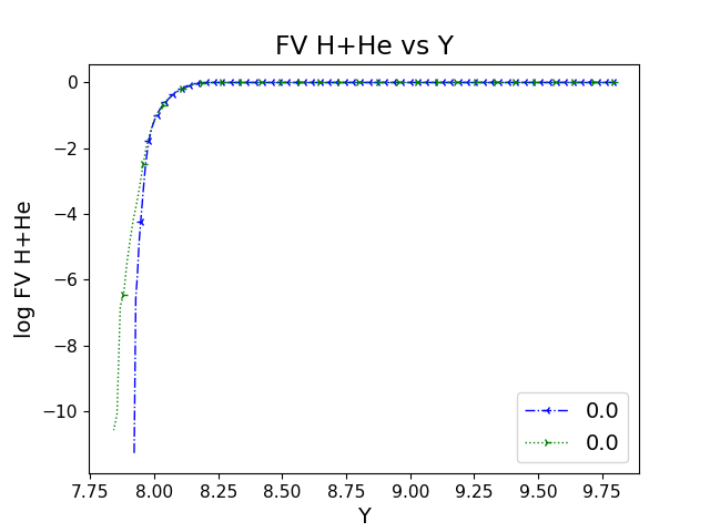
ppmpy.ppm.prof_compare(cases, ndump=None, yaxis_thing='FV H+He', ifig=None, num_type='ndump', labels=None, logy=True)

Compare profiles of quantities from multiple PPM Yprofile instances at a given time of nump number.

Parameters:

• cases (list) – list containing the Yprofile instances that you want to compare
• ndump (string or int, optional) – The filename, Ndump or time, if None it defaults to the last NDump. The default is None.
• yaxis_thing (string, optional) – What quantity to plot on the y-axis. The default is ‘FV H+He’
• ifig (int, optional) – Figure number. If None, chose automatically. The default is None.
• num_type (string, optional) – Designates how this function acts and how it interprets fname. If numType is ‘file’, this function will get the desired attribute from that file. If numType is ‘NDump’ function will look at the cycle with that nDump. If numType is ‘T’ or ‘time’ function will find the _cycle with the closest time stamp. The default is “ndump”.
• labels (list, optional) – List of labels; one for each of the cases. If None, labels are simply indices. The default is None.
• logy (boolean, optional) – Should the y-axis have a logarithmic scale? The default is True.

Examples

In [1]: from ppmpy import ppm
   ...: data_dir = '/data/ppm_rpod2/YProfiles/'
   ...: project = 'O-shell-M25'
   ...: ppm.set_YProf_path(data_dir+project)
   ...: 

In [5]: D2=ppm.yprofile('D2')
   ...: D1=ppm.yprofile('D1')
   ...: ppm.prof_compare([D2,D1],10,labels = ['D1','D2'])
   ...: 

ppmpy.ppm.set_YProf_path(path, YProf_fname='YProfile-01-0000.bobaaa')

Set path to location where YProfile directories can be found.

For example, set path to the swj/PPM/RUNS_DIR VOSpace directory as a global variable, so that it need only be set once during an interactive session; instances can then be loaded by refering to the directory name that contains YProfile files.

ppm.ppm_path: contains path ppm.cases: contains dirs in path that contain file with name YProf_fname usually used to determine dirs with YProfile files

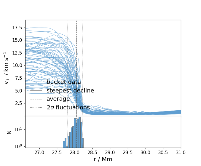
ppmpy.ppm.upper_bound_ut(data_path, dump_to_plot, hist_dump_min, hist_dump_max, r1, r2, ylims=None, derivative=False, silent=True)

Finds the upper convective boundary as defined by the steepest decline in tangential velocity.

Subpolot(1) plots the tangential velocity as a function of radius for a single dump and

displays the convective boundary

Subplot(2) plots a histogram of the convective boundaries for a range of dumps specified by

user and compares them to the selected dump

Plots Fig. 14 or 15 in paper: “Idealized hydrodynamic simulations of turbulent oxygen-burning shell convection in 4 geometry” by Jones, S.; Andrassy, R.; Sandalski, S.; Davis, A.; Woodward, P.; Herwig, F. NASA ADS: http://adsabs.harvard.edu/abs/2017MNRAS.465.2991J

Parameters:

• derivative (bool) – True = plot dut/dr False = plot ut
• dump_To_plot (int) – The file number of the dump you wish to plot
• = int (hist_dump_min/hist_dump_max) – Range of file numbers you want to use in the histogram
• r1/r2 (float) – This function will only search for the convective boundary in the range between r1/r2

Examples

In [1]: data_path = '/data/ppm_rpod2/RProfiles/AGBTP_M2.0Z1.e-5/F4/'
   ...: dump = 560; hist_dmin = dump - 1; hist_dmax = dump + 1
   ...: r_lim = (27.0, 30.5)
   ...: 

In [4]: ppm.upper_bound_ut(data_path,dump, hist_dmin, hist_dmax,r1 = r_lim[0],r2 = 31, derivative = False,ylims = [1e-3,19.])

ppmpy.ppm.v_evolution(cases, ymin, ymax, comp, RMS, sparse=1, markevery=25, ifig=12, dumps=[0, -1], lims=None)

Compares the time evolution of the max RMS velocity of different runs

Plots Fig. 12 in paper: “Idealized hydrodynamic simulations of turbulent oxygen-burning shell convection in 4 geometry” by Jones, S.; Andrassy, R.; Sandalski, S.; Davis, A.; Woodward, P.; Herwig, F. NASA ADS: http://adsabs.harvard.edu/abs/2017MNRAS.465.2991J

Parameters:

• cases (string array) – directory names that contain the runs you wish to compare assumes ppm.set_YProf_path was used, thus only the directory name is necessary and not the full path ex. cases = [‘D1’, ‘D2’]
• ymax (ymin,) – Boundaries of the range to look for vr_max in
• comp (string) – component that the velocity is in. option: ‘radial’, ‘tangential’
• RMS (string) – options: ‘min’, ‘max’ or ‘mean’. What aspect of the RMS velocity to look at
• dumps (int, optional) – Gives the range of dumps to plot if larger than last dump will plot up to last dump
• lims (array) – axes lims [xl,xu,yl,yu]

Examples

ppm.set_YProf_path(‘/data/ppm_rpod2/YProfiles/O-shell-M25/’,YProf_fname=’YProfile-01-0000.bobaaa’) ppm.v_evolution([‘D15’,’D2’,’D1’], 4., 8.,’max’,’radial’)

class ppmpy.ppm.yprofile(sldir='.', filename_offset=0, silent=True)

Data structure for holding data in the YProfile.bobaaa files.

Parameters:sldir (string) – which directory we are working in. The default is ‘.’.

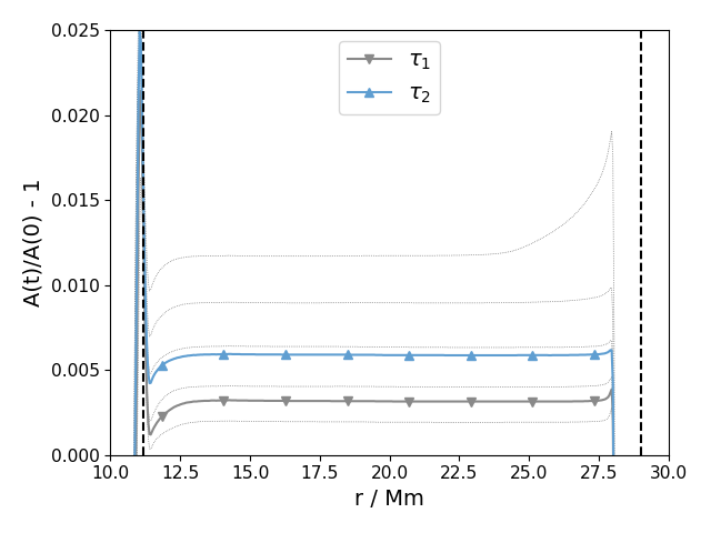
Aprof_time(tau, Nl, lims=None, save=False, silent=True, prefix='PPM', format='pdf', initial_conv_boundaries=True, lw=1.0, ifig=12)

Plots the same velocity profile at different times

Parameters:

• tau (array) – times to plot
• Nl (range) – Number of lines to plot, eg. range(0,10,1) would plot ten dotted contour lines for every minute from 0 to 10
• lims (list) – Limits for the plot, i.e. [xl,xu,yl,yu]. If None, the default values are used. The default is None.
• save (boolean) – Do you want the figures to be saved for each cycle? Figure names will be <prefix>-Vel-00000000001.<format>, where <prefix> and <format> are input options that default to ‘PPM’ and ‘pdf’. The default value is False.
• silent (boolean,optional) – Should plot display output?
• prefix (string) – see ‘save’ above
• format (string) – see ‘save’ above
• initial_conv_boundaries (logical) – plot vertical lines where the convective boundaries are initially, i.e. ad radbase and radtop from header attributes in YProfiles
• ifig (int) – figure number to plot into

Examples

In [1]: data_dir = '/data/ppm_rpod2/YProfiles/'
   ...: project = 'AGBTP_M2.0Z1.e-5'
   ...: ppm.set_YProf_path(data_dir+project)
   ...: 

In [4]: F4 = ppm.yprofile('F4')
   ...: F4.Aprof_time(np.array([807., 1399.]),range(0,30,5),lims =[10., 30.,0., 2.5e-2],silent = True)
   ...: 
The closest time is at Ndump = 559
The closest time is at Ndump = 970

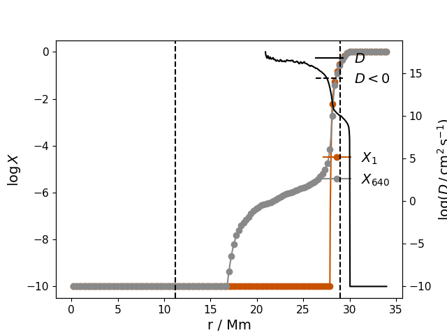
Dinv(fname1, fname2, fluid='FV H+He', numtype='ndump', newton=False, niter=3, debug=False, grid=False, FVaverage=False, tauconv=None, returnY=False, plot_Dlt0=True, silent=True, initial_conv_boundaries=True, approx_D=False, linelims=None, r0=None)

Solve inverted diffusion equation to see what diffusion coefficient profile would have been appropriate to mimic the mixing of species seen in the Yprofile dumps.

In the present version, we only solve for D in the region where ‘FV H+He’ is not 0 or 1 in dump fname 2.

Parameters:

• fname1,fname2 (int or float) – cycles from which to take initial and final abundance profiles for the diffusion step we want to mimic.
• fluid (string) – Which fluid do you want to track?
• numtype (string, optional) – Designates how this function acts and how it interprets fname. If numType is ‘file’, this function will get the desired attribute from that file. If numType is ‘NDump’ function will look at the cycle with that nDump. If numType is ‘T’ or ‘time’ function will find the _cycle with the closest time stamp. The default is “ndump”.
• newton (boolean, optional) – Whether or not to apply Newton-Raphson refinement of the solution for D. The default is False
• niter (int, optional) – If N-R refinement is to be done, niter is how many iterations to compute. The default is 3.
• grid (boolean, optional) – whether or not to show the axes grids. The default is False.
• FVaverage (boolean, optional) – Whether or not to average the abundance profiles over a convective turnover timescale. See also tauconv. The default is False.
• tauconv (float, optional) – If averaging the abundance profiles over a convective turnover timescale, give the convective turnover timescale (seconds). The default value is None.
• returnY (boolean, optional) – If True, return abundance vectors as well as radius and diffusion coefficient vectors The default is False.
• plot_Dlt0 (boolean, optional) – whether or not to plot the diffusion coefficient when it is negative
• approx_D (boolean, optional) – whether or not to plot an approximate diffusion coefficient for an area of the line
• linelims (range, optional) – limits of the radius to approximate diffusion coefficient default is none (whole vector)
• r0 (None, optional) – Start of exponential diffusion decay, necessary for approx_D

Returns:

• x (array) – radial co-ordinates (Mm) for which we have a diffusion coefficient
• D (array) – Diffusion coefficient (cm^2/s)

Examples

In [1]: data_dir = '/data/ppm_rpod2/YProfiles/'
   ...: project = 'AGBTP_M2.0Z1.e-5'
   ...: ppm.set_YProf_path(data_dir+project)
   ...: 

In [4]: F4 = ppm.yprofile('F4')
   ...: res = F4.Dinv(1,640)
   ...: 

Dov(r0, D0, f, fname=1)

Calculate and plot an exponentially decaying diffusion coefficient given an r0, D0 and f.

Dov is given by the formula D0*exp(-2*(r-r0)/f*Hp)

Parameters:

• r0 (float) – radius (Mm) at which the decay will begin
• D0 (float) – diffusion coefficient at r0
• f (float) – what f-value (parameter, where f*Hp is the e-folding length of the diffusion coefficient) should we decay with?
• fname (int) – which dump do you want to take r and P from?

Returns:

• r (array) – radial co-ordinates (Mm) for which we have a diffusion coefficient the decays exponentially
• D (array) – Exponentially decaying diffusion coefficient (cm^2/s)

Dov2(r0, D0, f1=0.2, f2=0.05, fname=1, silent=True)

Calculate and plot an 2-parameter exponentially decaying diffusion coefficient given an r0, D0 and f1 and f2.

Dov is given by the formula: D = 2. * D0 * 1. / (1. / exp(-2*(r-r0)/f1*Hp) + 1. / exp(-2*(r-r0)/f2*Hp))

Parameters:

• r0 (float) – radius (Mm) at which the decay will begin
• D0 (float) – diffusion coefficient at r0
• f1,f2,A (float) – parameters of the model
• fname (int) – which dump do you want to take r and P from?

Returns:

• r (array) – radial co-ordinates (Mm) for which we have a diffusion coefficient the decays exponentially
• D (array) – Exponentially decaying diffusion coefficient (cm^2/s)

Dsolve(fname1, fname2, fluid='FV H+He', numtype='ndump', newton=False, niter=3, debug=False, grid=False, FVaverage=False, tauconv=None, returnY=False)

Solve inverse diffusion equation sequentially by iterating over the spatial domain using a lower boundary condition (see MEB’s thesis, page 223, Eq. B.15).

Parameters:

• fname1,fname2 (int or float) – cycles from which to take initial and final abundance profiles for the diffusion step we want to mimic.
• fluid (string) – Which fluid do you want to track? numtype : string, optional Designates how this function acts and how it interprets fname. If numType is ‘file’, this function will get the desired attribute from that file. If numType is ‘NDump’ function will look at the cycle with that nDump. If numType is ‘T’ or ‘time’ function will find the _cycle with the closest time stamp. The default is “ndump”.
• newton (boolean, optional) – Whether or not to apply Newton-Raphson refinement of the solution for D. The default is False
• niter (int, optional) – If N-R refinement is to be done, niter is how many iterations to compute. The default is 3.
• grid (boolean, optional) – whether or not to show the axes grids. The default is False.
• FVaverage (boolean, optional) – Whether or not to average the abundance profiles over a convective turnover timescale. See also tauconv. The default is False.
• tauconv (float, optional) – If averaging the abundance profiles over a convective turnover timescale, give the convective turnover timescale (seconds). The default value is None.
• returnY (boolean, optional) – If True, return abundance vectors as well as radius and diffusion coefficient vectors The default is False.

Returns:

• x (array) – radial co-ordinates (Mm) for which we have a diffusion coefficient
• D (array) – Diffusion coefficient (cm^2/s)

Dsolvedown(fname1, fname2, fluid='FV H+He', numtype='ndump', newton=False, niter=3, debug=False, grid=False, FVaverage=False, tauconv=None, returnY=False, smooth=False, plot_Dlt0=True, sinusoidal_FV=False, log_X=True, Xlim=None, Dlim=None, silent=True, showfig=True)

Solve diffusion equation sequentially by iterating over the spatial domain inwards from the upper boundary.

Parameters:

• fname1,fname2 (int or float) – cycles from which to take initial and final abundance profiles for the diffusion step we want to mimic.
• fluid (string) – Which fluid do you want to track?
• numtype (string, optional) – Designates how this function acts and how it interprets fname. If numType is ‘file’, this function will get the desired attribute from that file. If numType is ‘NDump’ function will look at the cycle with that nDump. If numType is ‘T’ or ‘time’ function will find the _cycle with the closest time stamp. The default is “ndump”.
• newton (boolean, optional) – Whether or not to apply Newton-Raphson refinement of the solution for D. The default is False
• niter (int, optional) – If N-R refinement is to be done, niter is how many iterations to compute. The default is 3.
• grid (boolean, optional) – whether or not to show the axes grids. The default is False.
• FVaverage (boolean, optional) – Whether or not to average the abundance profiles over a convective turnover timescale. See also tauconv. The default is False.
• tauconv (float, optional) – If averaging the abundance profiles over a convective turnover timescale, give the convective turnover timescale (seconds). The default value is None.
• returnY (boolean, optional) – If True, return abundance vectors as well as radius and diffusion coefficient vectors The default is False.
• smooth (boolean, optional) – Smooth the abundance profiles with a spline fit, enforcing their monotonicity. Only works for FV H+He choice of fluid
• plot_Dlt0 (boolean, optional) – whether or not to plot D where it is <0 the default value is True

Returns:

• x (array) – radial co-ordinates (Mm) for which we have a diffusion coefficient
• D (array) – Diffusion coefficient (cm^2/s)

Dsolvedownexp(fname1, fname2, fluid='FV H+He', numtype='ndump', newton=False, niter=3, debug=False, grid=False, FVaverage=False, tauconv=None, returnY=False)

Solve diffusion equation sequentially by iterating over the spatial domain inwards from the upper boundary. This version of the method is explicit.

Parameters:

• fname1,fname2 (int or float) – cycles from which to take initial and final abundance profiles for the diffusion step we want to mimic.
• fluid (string) – Which fluid do you want to track?
• numtype (string, optional) – Designates how this function acts and how it interprets fname. If numType is ‘file’, this function will get the desired attribute from that file. If numType is ‘NDump’ function will look at the cycle with that nDump. If numType is ‘T’ or ‘time’ function will find the _cycle with the closest time stamp. The default is “ndump”.
• newton (boolean, optional) – Whether or not to apply Newton-Raphson refinement of the solution for D. The default is False
• niter (int, optional) – If N-R refinement is to be done, niter is how many iterations to compute. The default is 3.
• grid (boolean, optional) – whether or not to show the axes grids. The default is False.
• FVaverage (boolean, optional) – Whether or not to average the abundance profiles over a convective turnover timescale. See also tauconv. The default is False.
• tauconv (float, optional) – If averaging the abundance profiles over a convective turnover timescale, give the convective turnover timescale (seconds). The default value is None.
• returnY (boolean, optional) – If True, return abundance vectors as well as radius and diffusion coefficient vectors The default is False.

Returns:

• x (array) – radial co-ordinates (Mm) for which we have a diffusion coefficient
• D (array) – Diffusion coefficient (cm^2/s)

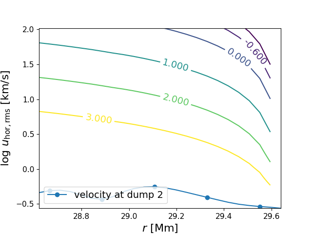
Richardson_plot(fname1=0, fname2=2, R_low=None, R_top=None, do_plots=False, logRi_levels=[-1.0, -0.6, 0.0, 1.0, 2.0, 3.0], ylim_max=2.02, compressible_fluid=True, plot_type=0, ifig=101)

Make a plot of radius vs tangential velocity in the vicinity of the boundary and draw on lines of constant Richardson number. Compared to the function that produced Fig. 9 of Woodward+ (2015) this one takes into account the compressibility of the gas. Several bugs have been removed, too.

Parameters:

• fname1 (int) – Which dump do you want to take the stratification from?
• fname2 (int) – Which dump do you want to take the velocities from?
• R_low (float) – The minimum radius in the plot. If invalid or None it will be set to R_top - 1.
• R_top (float) – Radius of top of convection zone. If invalid or None it will be set to the radius at which FV H+He = 0.9.
• do_plots (logical) – Do you want to do some intermittent plotting?
• logRi_levels (list, optional) – Values of Ri for which to draw contours.
• ylim_max (float) – Max of ylim (min is automatically determined) in the final plot.
• compressible_fluid (logical) – You can set it to False to use the Richardson criterion for an incompressible fluid.
• plot_type (int) – plot_type = 0: Use a variable lower endpoint and a fixed upper endpoint of the radial interval, in which Ri is calculated. Ri is plotted for a range of assumed velocity differences with respect to the upper endpoint. plot_type = 1: Compute Ri locally assuming that the local velocities vanish on a certain length scale, which is computed from the radial profile of the RMS horizontal velocity.
• ifig (int) – Figure number for the Richardson plot (a new window must be opened).

Examples

In [1]: data_dir = '/data/ppm_rpod2/YProfiles/'
   ...: project = 'AGBTP_M2.0Z1.e-5'
   ...: ppm.set_YProf_path(data_dir+project)
   ...: 

In [4]: F4 = ppm.yprofile('F4')
   ...: F4.Richardson_plot()
   ...: 
R_top set to 29.639.
R_low centred on the cell nearest to R_top - 1: R_low = 28.621.

boundary_radius(cycles, r_min, r_max, var='vxz', criterion='min_grad', var_value=None)

Calculates the boundary of the yprofile.

Parameters:

• cycles (range) – range of yprofiles to calculate boundary for
• r_min (float) – min rad to look for boundary
• r_max (float) – max rad to look for boundary

Returns:

rb – boundary of cycles

Return type:

array

computeData(attri, fname, numtype='ndump', silent=False, **kwargs)

Method for computing data not in Yprofile file

Parameters:

• attri (str) – What you are looking for
• fname (int) – what dump or time you are look for attri at time or dump specifies by numtype.
• numtype (str, optional) – ‘ndump’ or ‘time’ depending on which you are looking for

Returns:

attri – An array for the attirbute you are looking for

Return type:

array

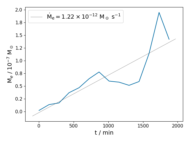
entrainment_rate(cycles, r_min, r_max, var='vxz', criterion='min_grad', offset=0.0, integrate_both_fluids=False, integrate_upwards=False, show_output=True, ifig0=1, silent=True, mdot_curve_label=None, file_name=None, return_time_series=False)

Function for calculating entrainment rates.

Parameters:

• cycles (range) – cycles to get entrainment rate for
• r_min (float) – minimum radius to look for boundary
• r_max (float) – maximum radius to look for boundary

Examples

In [1]: data_dir = '/data/ppm_rpod2/YProfiles/'
   ...: project = 'AGBTP_M2.0Z1.e-5'
   ...: ppm.set_YProf_path(data_dir+project)
   ...: 

In [4]: F4 = ppm.yprofile('F4')
   ...: dumps = np.array(range(0,1400,100))
   ...: F4.entrainment_rate(dumps,27.7,28.5)
   ...: 
Out[6]: 1.22407890578549e-12

findFile(FName, numType='FILE', silent=False)

Function that finds the associated file for FName when Fname is time or NDump.

Parameters:

• FName (string) – The name of the file, Ndump or time we are looking for.
• numType (string, optional) – Designates how this function acts and how it interprets FName. If numType is ‘file’, this function will get the desird attribute from that file. If numType is ‘NDump’ function will look at the cycle with that nDump. If numType is ‘T’ or ‘time’ function will find the cycle with the closest time stamp. The default is “FILE”.

Returns:

FName – The number corresponding to the file.

Return type:

int

get(attri, fname=None, numtype='ndump', resolution='H', silent=True, **kwargs)

Method that dynamically determines the type of attribute that is passed into this method. Also it then returns that attribute’s associated data.

Parameters:

• attri (string) – The attribute we are looking for.
• fname (string, optional) – The filename, Ndump or time, if None it defaults to the last NDump. The default is None.
• numtype (string, optional) – Designates how this function acts and how it interprets fname. If numType is ‘file’, this function will get the desired attribute from that file. If numType is ‘NDump’ function will look at the cycle with that nDump. If numType is ‘T’ or ‘time’ function will find the _cycle with the closest time stamp. The default is “ndump”.
• Resolution (string, optional) – Data you want from a file, for example if the file contains two different sized columns of data for one attribute, the argument ‘a’ will return them all, ‘h’ will return the largest, ‘l’ will return the lowest. The default is ‘H’.

getCattrs()

returns the list of cycle attributes

getColData(attri, FName, numType='ndump', resolution='H', cycle=False, silent=False)

Method that returns column data.

Parameters:

• attri (string) – Attri is the attribute we are loking for.
• FName (string) – The name of the file, Ndump or time we are looking for.
• numType (string, optional) – Designates how this function acts and how it interprets FName. If numType is ‘file’, this function will get the desired attribute from that file. If numType is ‘NDump’ function will look at the cycle with that nDump. If numType is ‘T’ or ‘time’ function will find the _cycle with the closest time stamp. The default is “ndump”.
• Resolution (string, optional) – Data you want from a file, for example if the file contains two different sized columns of data for one attribute, the argument ‘a’ will return them all, ‘H’ will return the largest, ‘l’ will return the lowest. The defalut is ‘H’.
• cycle (boolean, optional) – Are we looking for a cycle or column attribute. The default is False.

Returns:

A Datalist of values for the given attribute.

Return type:

list

Notes

To ADD: options for a middle length of data.

getCycleData(attri, FName=None, numType='ndump', Single=False, resolution='H', silent=False)

Method that returns a Datalist of values for the given attribute or a single attribute in the file FName.

Parameters:

• attri (string) – What we are looking for.
• FName (string, optional) – The filename, Ndump or time, if None it defaults to the last NDump. The default is None.
• numType (string, optional) – Designates how this function acts and how it interprets FName. If numType is ‘file’, this function will get the desired attribute from that file. If numType is ‘NDump’ function will look at the cycle with that nDump. If numType is ‘T’ or ‘time’ function will find the _cycle with the closest time stamp. The default is “ndump”.
• Single (boolean, optional) – Determining whether the user wants just the Attri contained in the specified ndump or all the dumps below that ndump. The default is False.
• Resolution (string, optional) – Data you want from a file, for example if the file contains two different sized columns of data for one attribute, the argument ‘a’ will return them all, ‘h’ will return the largest, ‘l’ will return the lowest. The defalut is ‘H’.

Returns:

A Datalist of values for the given attribute or a single attribute in the file FName.

Return type:

list

getDCols()

returns the list of column attributes

getHattrs()

returns the list of header attributes

getHeaderData(attri, silent=False)

Method returns header attributes.

Parameters:attri (string) – The name of the attribute. Returns:data – Header data that is associated with the attri. Return type:string or integer

Notes

To see all possable options in this instance type instance.getHattrs().

get_mass_fraction(fname, resolution)

Get mass fraction profile of fluid ‘fluid’ at fname with resolution ‘resolution’.

ndumpDict(fileList, filename_offset=0)

Method that creates a dictionary of Filenames with the associated key of the filename’s Ndump.

Parameters:fileList (list) – A list of yprofile filenames. Returns:dictionary – the filename, ndump dictionary Return type:dict

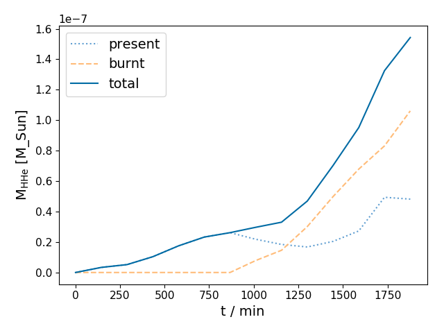
plot_entrainment_rates(dumps, r1, r2, fit=False, fit_bounds=None, save=False, lims=None, ifig=4, Q=3.1146379199999996e-49, RR=8.3144598, amu=1.66054e-51, airmu=1.39165, cldmu=0.725, fkair=0.203606102635, fkcld=0.885906040268, AtomicNoair=6.65742024965, AtomicNocld=1.34228187919)

Plots entrainment rates for burnt and unburnt material

Parameters:

• data_path (str) – data path
• r1 (float) – This function will only search for the convective boundary in the range between r1/r2
• r2 (float) –
• fit (boolean, optional) – show the fits used in finding the upper boundary
• fit_bounds (array) – The time to start and stop the fit for average entrainment rate units in minutes
• save (bool, optional) – save the plot or not
• lims (list, optional) – axes lims [xl,xu,yl,yu]

Examples

In [1]: data_dir = '/data/ppm_rpod2/YProfiles/'
   ...: project = 'AGBTP_M2.0Z1.e-5'
   ...: ppm.set_YProf_path(data_dir+project)
   ...: 

In [4]: F4 = ppm.yprofile('F4')
   ...: dumps = np.array(range(0,1400,100))
   ...: F4.plot_entrainment_rates(dumps,27.7,28.5)
   ...: 

prof_time(fname, yaxis_thing='vY', num_type='ndump', logy=False, radbase=None, radtop=None, ifig=101, ls_offset=0, label_case=' ', markevery=None, **kwargs)

Plot the time evolution of a profile from multiple dumps of the same run (…on the same figure).

Velocities ‘v’, ‘vY’ and/or ‘vXZ’ may also be plotted.

Parameters:

• fname (int or list) – Cycle or list of cycles to plot. Could also be time in minutes (see num_type).
• yaxis_thing (string) – What should be plotted on the y-axis? In addition to the dcols quantities, you may also choose ‘v’, ‘vY’, and ‘vXZ’ – the RMS ‘total’, radial and tangential velocities. The default is ‘vY’.
• logy (boolean) – Should the velocity axis be logarithmic? The default value is False
• radbase (float) – Radii of the base of the convective region, respectively. If not None, dashed vertical lines will be drawn to mark these boundaries. The default value is None.
• radtop (float) – Radii of the top of the convective region, respectively. If not None, dashed vertical lines will be drawn to mark these boundaries. The default value is None.
• num_type (string, optional) – Designates how this function acts and how it interprets fname. If numType is ‘file’, this function will get the desired attribute from that file. If numType is ‘NDump’ function will look at the cycle with that nDump. If numType is ‘T’ or ‘time’ function will find the _cycle with the closest time stamp. The default is “ndump”.
• ifig (integer) – figure number
• ls_offset (integer) – linestyle offset for argument in utils.linestyle for plotting more than one case
• label_case (string) – optional extra label for case

Examples

In [1]: from ppmpy import ppm
   ...: data_dir = '/data/ppm_rpod2/YProfiles/'
   ...: project = 'O-shell-M25'
   ...: ppm.set_YProf_path(data_dir+project)
   ...: 

In [5]: D2 = ppm.yprofile('D2')
   ...: D2.prof_time([0,5,10],logy=False,num_type='time',ifig=78)
   ...: 

readTop(atri, filename, stddir='./')

Private routine that Finds and returns the associated value for attribute in the header section of the file.

Input: atri, what we are looking for. filename where we are looking. StdDir the directory where we are looking, Defaults to the working Directory.

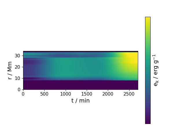
spacetime_diagram(var_name, nt, fig, tlim=None, rlim=None, vlim=None, logscale=True, cmap='viridis', aspect=0.3333333333333333, zero_intervals=None, patience0=5, patience=30, **kwargs)

Creates a spacetime diagram.

Parameters:

• var_name (str) – variable to plot
• nt (int) – size of time vector, t = np.linspace(t0,tf,nt)

Examples

In [1]: data_dir = '/data/ppm_rpod2/YProfiles/'
   ...: project = 'AGBTP_M2.0Z1.e-5'
   ...: ppm.set_YProf_path(data_dir+project)
   ...: 

In [4]: F4 = ppm.yprofile('F4')
   ...: import matplotlib.pyplot as plt
   ...: fig2 = plt.figure(19)
   ...: F4.spacetime_diagram('Ek',5,fig2)
   ...: 
vlim = [1.879e+06, 2.851e+16]

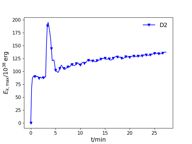
tEkmax(ifig=None, label=None, save=False, prefix='PPM', format='pdf', logy=False, id=0)

Plot maximum kinetic energy as a function of time.

Parameters:

• ifig (int, optional) – Figure number. If None, chose automatically. The default is None.
• label (string, optional) – Label for the model The default is None.
• save (boolean, optional) – Do you want the figures to be saved for each cycle? Figure names will be <prefix>-t-EkMax.<format>, where <prefix> and <format> are input options that default to ‘PPM’ and ‘pdf’. The default value is False.
• prefix (string, optional) – see ‘save’ above
• format (string, optional) – see ‘save’ above
• logy (boolean, optional) – Should the y-axis have a logarithmic scale? The default is False
• id (int, optional) – An id for the model, which esures that the lines are plotted in different colours and styles. The default is 0

Examples

In [1]: data_dir = '/data/ppm_rpod2/YProfiles/'
   ...: project = 'O-shell-M25'
   ...: ppm.set_YProf_path(data_dir+project)
   ...: 

In [4]: D2 = ppm.yprofile('D2')
   ...: D2.tEkmax(ifig=77,label='D2',id=0)
   ...: 

tvmax(ifig=None, label=None, save=False, prefix='PPM', format='pdf', logy=False, id=0)

Plot maximum velocity as a function of time.

Parameters:

• ifig (int, optional) – Figure number. If None, chose automatically. The default is None.
• label (string, optional) – Label for the model The default is None.
• save (boolean) – Do you want the figures to be saved for each cycle? Figure names will be <prefix>-t-vMax.<format>, where <prefix> and <format> are input options that default to ‘PPM’ and ‘pdf’. The default value is False.
• prefix (string) – see ‘save’ above
• format (string) – see ‘save’ above
• logy (boolean, optional) – Should the y-axis have a logarithmic scale? The default is False
• id (int, optional) – An id for the model, which esures that the lines are plotted in different colours and styles. The default is 0

Examples

In [1]: data_dir = '/data/ppm_rpod2/YProfiles/'
   ...: project = 'O-shell-M25'
   ...: ppm.set_YProf_path(data_dir+project)
   ...: 

In [4]: D2 = ppm.yprofile('D2')
   ...: D2.tvmax(ifig=11,label='D2',id=0)
   ...: 

vaverage(vi='v', transient=0.0, sparse=1, showfig=False)

plots and returns the average velocity profile for a given orientation (total, radial or tangential) over a range of dumps and excluding an initial user-specified transient in seconds.

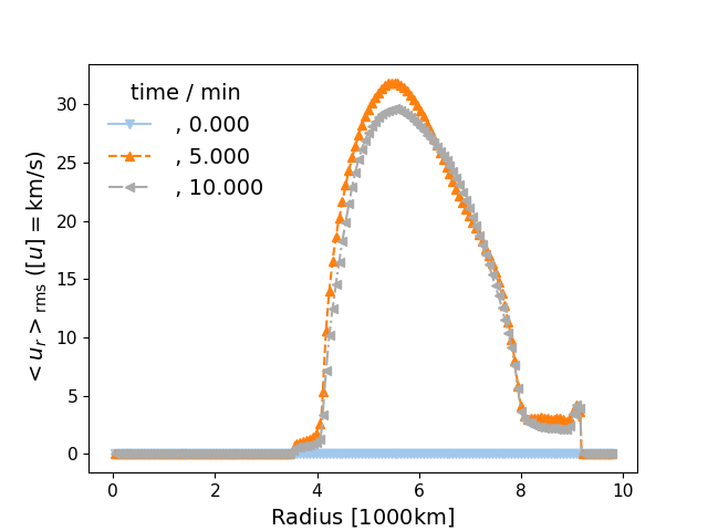
vprof_time(dumps, Np, comp='r', lims=None, save=False, prefix='PPM', format='pdf', initial_conv_boundaries=True, lw=1.0, ifig=12)

Plots the same velocity profile at different times

Parameters:

• dumps (array) – dumps to plot
• Np (int) – This function averages over a range of Np points centered at the dump number, preferable an even number or else the range will not be centered around the dump number
• comp (str) – ‘r’ ‘t’ or ‘tot’ for the velocity component that will be plotted see vprof for comparing all three
• lims (list) – Limits for the plot, i.e. [xl,xu,yl,yu]. If None, the default values are used. The default is None.
• save (bool) – Do you want the figures to be saved for each cycle? Figure names will be <prefix>-Vel-00000000001.<format>, where <prefix> and <format> are input options that default to ‘PPM’ and ‘pdf’. The default value is False.
• prefix (str) – see ‘save’ above
• format (string) – see ‘save’ above
• initial_conv_boundaries (bool, optional) – plot vertical lines where the convective boundaries are initially, i.e. ad radbase and radtop from header attributes in YProfiles
• ifig (int) – figure number to plot into

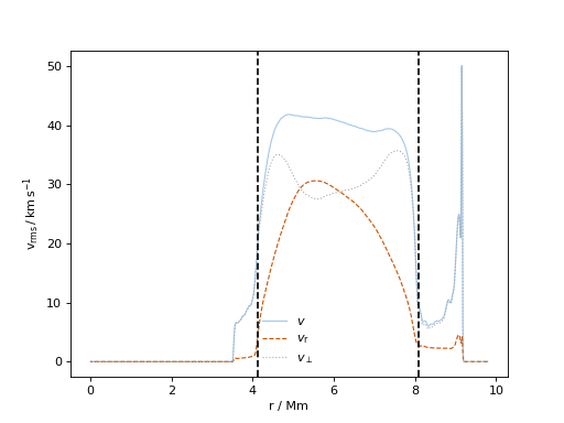
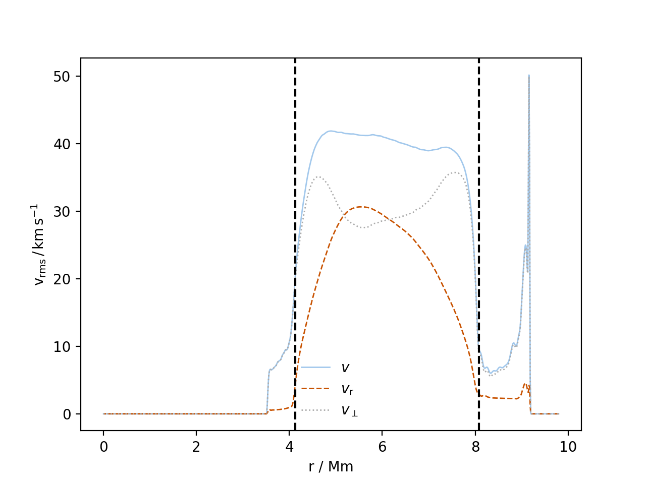
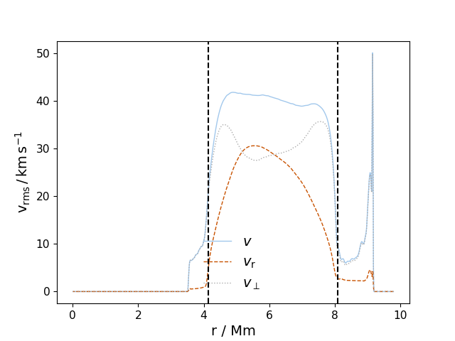
vprofs(fname, fname_type='discrete', log_logic=False, lims=None, save=False, prefix='PPM', format='pdf', initial_conv_boundaries=True, lw=1.0, label=True, ifig=11, which_to_plot=[True, True, True], run=None)

Plot velocity profiles v_tot, v_Y and v_XZ for a given cycle number or list of cycle numbers (fname). If a list of cycle number is given, separate figures are made for each cycle. If one wishes to compare velocity profiles for two or more cycles, see function vprof_time.

Parameters:

• fname (int or list) – Cycle number or list of cycle numbers to plot
• fname_type (string) – ‘discrete’ or ‘range’ whether to average over a range to find velocities or plot entries discretely default is ‘discrete’
• log_logic (boolean) – Should the velocity axis be logarithmic? The default value is False
• lims (list) – Limits for the plot, i.e. [xl,xu,yl,yu]. If None, the default values are used. The default is None.
• save (boolean) – Do you want the figures to be saved for each cycle? Figure names will be <prefix>-Vel-00000000001.<format>, where <prefix> and <format> are input options that default to ‘PPM’ and ‘pdf’. The default value is False.
• prefix (string) – see ‘save’ above
• format (string) – see ‘save’ above
• initial_conv_boundaries (logical) – plot vertical lines where the convective boundaries are initially, i.e. ad radbase and radtop from header attributes in YProfiles
• lw (float, optional) – line width of the plot
• label (string, optional) – label for the line, if multiple models plotted
• which_to_plot (boolean array, optional) – booleans as to whether to plot v_tot v_Y and v_XZ respectively True to plot
• run (string, optional) – the name of the run

Examples

In [1]: data_dir = '/data/ppm_rpod2/YProfiles/'
   ...: project = 'O-shell-M25'
   ...: ppm.set_YProf_path(data_dir+project)
   ...: 

In [4]: D2 = ppm.yprofile('D2')
   ...: D2.vprofs(100,ifig = 111)
   ...: